Computational Simulations-Optimization of UHMWPE Knee Arthroplasty Linear Abrasive Wear

Abstract

Today, total knee arthroplasty (TKA) implants represent one of the most highly demanded prosthetic devices in the biomechanical and orthopedic surgical industries. Computational simulation models and algorithms for abrasive linear wear in total knee arthroplasty (TKA) are developed and presented for ultra-high-molecular-weight polyethylene (UHMWPE) components. This material is widely used for TKA implants. The implemented mathematical framework is based on the classical Archard’s wear model, modified to account for linear abrasive wear specific to TKA applications. The algorithms corresponding to both integer and integral formulations are described. For computational intelligence simulations, experimental data selected from the literature, including both in vitro and in vivo studies, are incorporated within the programming environment. Three-dimensional image-processing and computational simulation software are developed using graphical and interior optimization techniques. Linear wear results from million-cycle (Mc) simulations, presented as numerical datasets and three-dimensional image-processing graphs, are demonstrated and compared with data reported in the literature. Relevant biotribology, biomaterials, and biomedical applications related to total knee arthroplasty (TKA), including clinical and manufacturing aspects, are briefly discussed.

1. Introduction and Objectives

The biomechanics of total knee arthroplasty (TKA) are inherently complex due to several contributing factors. Foremost among these is the knee’s primary function of supporting total body weight as part of the third major biomechanical system of human anatomy [1,2]. The first system comprises the head and neck, the second includes the thorax, abdomen, spine, and hip, and the third consists of the knee, legs, and feet. The second reason is the biodynamics of walking and movement, which require balance and support for the body’s center of gravity. The third, and equally important, reason is that the articulations of the knee, ankle, and feet constitute a critical biomechanical system essential for walking and other fundamental movements of daily life. Complementary reasons include the aging and degeneration of cartilage and bone, and the probability of injuries from forced movements. All of them are mutually synergistic and constitute an interrelated biomechanical system [1-4]. In other words, premature degeneration of the knee joint cartilage can lead to bone damage, resulting in joint instability and loss of balance, which in turn limits or impedes normal movement dynamics. It should be noted that, histologically, cartilage cells lack regenerative capacity, unlike elastic fibers in the skin; although stem cell–based approaches are under investigation, they are beyond the scope of this study. That is, once growth and development are complete, an individual possesses a fixed number of elastic fibers in the skin and cartilage cells. The function of the menisci, which biomechanically resembles that of the intervertebral discs in terms of load damping, demonstrates a natural design adapted to withstand high biodynamic loads and enforced movements. What does the menisci is to spread the loads created by femur condyle. Furthermore, the second biomechanical system, in particular the hip articulation, can be damaged by forced/biased movements and biomechanical abnormal load distributions at the knee joint. This brief discussion provides a fundamental understanding of the complications that may arise in surgical pathology and biomechanical disorders of the knee joint.

On the other hand, knee injuries, joint traumatological conditions, and concomitant rheumatological or infectious diseases create a high medical and industrial demand. Consequently, the economic cost [1-8] is substantial for public, private, and mixed healthcare systems in many countries. Therefore, investigation of TKA prostheses for reliability and high durability is among the current priorities in the biomedical industry. Biomathematical studies using optimization modeling address the prediction of wear and the durability of TKA prostheses. An additional issue is the large number of model variants and the diversity of testing laboratories. This implies the requirement for standard methods, both experimental and theoretical-modelling. In this study, the most commonly applied ISO-related standards [1-11] are prioritized to meet the study objectives. For the femoral component (Figure 1), cobalt-chrome is predominantly used, with several variants available [3,11].

Previous studies have typically employed 2D finite element analyses; however, the present study focuses primarily on 3D graphical optimization. Those are made exclusively in FE [3,11], or with/without in-vitro/in-vivo cadaveric comparisons [12-18]. Since in vivo studies usually present linear wear data in mm/year or mg/year (the latter is generally for volume wear), and in vitro studies are expressed in mm/Mc, it is necessary to approximate the average Mc that a standard patient completes in a year [16]. In this study, calculations were estimated at approximately 2 Mc per year [16]. The specifications of Archard’s laws (fundamental, differential, and modified), along with standard units, are often not provided with detailed explanations or variants for most researchers [12-18]. Additionally, the utility of the presented algorithms for implementation in finite element or simpler simulations should be clearly detailed to allow other researchers to set up options efficiently. This article presents solutions to these hurdles in the simplest terms. Additionally, the 3D innovative Graphical Optimization charts that are shown/developed constitute a complement to other literature graphics.

The mathematical equations and models used are for Linear Abrasive Wear (in mm) without Creep and Lubrication Factors [3] at this stage. For Volume Wear (in mm³), the Finite Elements Method is widely applied [1-11]. Compared to the Finite Elements method, this direct algorithm implementation in 2D–3D graphical optimization offers some advantages. The first advantage is that it is less labor-intensive and requires less time than finite element analysis. The second is that implementing multiple algorithms simultaneously within a single program is straightforward and allows for direct comparisons. In brief, the rapid adaptability of the programming algorithm provides a clear advantage over the finite element method, both as a laboratory tool and as an initial approximation. Moreover, this algorithmic technique can be implemented alongside the finite element method or used to generate a database for further finite element applications.

Therefore, the computational model incorporates innovations and improvements over previous models for several reasons. First, it comprises the entire published range of the linear wear constant, Kw [3], namely approximately [2.20 × 10⁻⁷, 10⁻⁶]. In several figures, the values of Kw are multiplied by10⁻³ due to the software unit settings for 3D images. Second, it plots in 2D–3D the standard load range, the computational calculations (vectors) for the load range, and the computational calculations (vectors) for the K_w range. Third, the million cycles (Mc) range is set computationally in multiple 2D–3D graphics, in pattern with those loads and Kw ranges (Figure 2). Another advantage is the use of 3D surfaces to identify optimal settings when preparing for finite element analysis.

Table 1:

Selected Dataset used for simulations and optimization software. Disclaimer: Some variants were applied for trial programs and images. Note: In the figures, the K_w axis values are often multiplied by10⁻³. Figure 1, Figure 2, Figure 3, Figure 4, Figure 5, Figure 6, Figure 7 and Figure 8 present extensive image-processing data.

Selected Dataset Used for Simulations
Parameter and Units	Interval or Magnitude Software Implemented	References	Comments
Load (N)	[2000, 2300–2600]	[1, 11, 19-21]	Standard magnitude, usually agreed upon by most authors.
Sliding Distance (mm)	60	[10]	ISO Standard, it varies according to studies.
KW (mm3/(N × mm)	[2.20 × 10−7, 10−6]	[3, 19-21]	The constant KW has different values in the literature. An interval is implemented that comprises most published magnitudes.
Load Surface (mm2)	[400, 800]	[19-21]	This varies significantly across publications.
Cycles Number (in M (millions)) notation standard: Mc	[1, 5] Image processing is shown for [1, 5] Mc	[1-11, 13-34]	It is usually presented in most books and papers as a dataset from 1 M to 5 M. Most authors present predictions and calculations for 1–5 Mc.
Implemented: KW (mm3/(N × mm)) × 10−3 According to (4)	[2.20 × 10−10, 10−9]	[3]	KW has a different magnitude according to authors [3], and some researchers propose values of KW, for example [19-21].
Poisson ratio, Elastic modulus, Density for UHMWPE	Not implemented, Exclusively illustrative UHWMPE: Young’s modulus 463 MPa, Poisson’s ratio 0.46, density 960 kg/m3 [19-21].	[19-21]	N/A for the algorithms that are programmed.

Note: In the figures, the values/range of Kw are usually multiplied by 10−3 because all the units are set in mm in the software.

Table 2:

Selected Dataset literature and Author sources for Table 1. It is very frequent to find different magnitude orders for K_W in the literature. The current term for this constant is the wear coefficient. Recently, a dimensionless constant, referred to as the wear factor, has been applied in new models.

Dataset Reference Sources Discussed
Parameter and Units Criteria	Linear-Wear Details and References for Software Implemented	Justification
Load (N)	[1, 11, 19-21] Loads depend on the ISO experimental system used in many cases. Therefore, magnitudes are not standard. The most common interval reported in the literature is [2000, 2300–2600]. However, some Authors [21] apply loads of 3000 N, which is considered too high. In the same way [10], the magnitude of 1200 N is too low.	Standard magnitude, usually agreed upon by most authors.
Sliding Distance (mm)	[10] Sliding distance varies in the literature. The most frequent magnitude was selected. Moreover, the dataset choice comprised exclusively values referring to ISO standards. The interval in [10] is approximately [38.7, 83.7] mm.	ISO Standard, it varies. It is necessary to select the most frequent interval.
KW (mm3/(N × mm)	[3, 21-23] It is very frequent to find different magnitude orders for KW in the literature. This constant is currently referred to as the wear factor, corresponding to Archard model first generation models. Recently, a dimensionless constant called the wear coefficient has been applied in new second generation cross-shear models.	The [3] range is applied for software.
Load Surface (mm2)	[19-21] The magnitude value intervals comprise the most frequent in the literature.	[1] shows standard coronal size and loads.
Cycles Number (in M (millions)) notation standard: Mc	[1-11, 13-34] In the literature, results using Mc are usually shown for 1 to 5. Ms is the most common form for presenting linear and volumetric wear.	Usually, a dataset from 1 Mc to 5 Mc is presented. In Figure 7, a 1–6 Mc composition is shown with numerical results.
Implemented: KW (mm3/(N × mm)) × 10−3 According to [3]	[3] Both the wear factor (dimensional) and the recent wear coefficient (adimensional) for new models show differences in the literature. Reference [3] presents extensive data showing a variation of one order of magnitude.	Table 1 interval is considered a sufficiently confident interval that comprises almost all authors’ publications.

In summary, following the introduction of these fundamental concepts, the study focuses on computational intelligence-based optimization of biomechanical models and presents practical numerical and image processing results, primarily for ultra-high molecular weight polyethylene (UHMWPE).

1.1. The Biomechanical Concepts of Knee Articulation

Figure 1 illustrates the basic knee biomechanical system following TKA implantation, including its components and movement concepts. In normal life, the knee articulation supports biomechanical stress, loads, flexions, extensions, torsions, rotations, and more complicated movements. Furthermore, the knee is not solely composed of the joint itself; the cruciate ligaments, as well as the medial, lateral, and other surrounding ligaments, form a highly complex articulated biosystem. This contributes to the relatively high incidence and prevalence of knee biomechanical pathologies. Sports activities increase the risk of injury, and in that field, the knee articulation supports loads and extreme movements continuously [1-2, 5-6, 10]. The sports medicine specialization for the knee is a branch with deep knowledge and applications.

1.2. Biomechanical Knee Implants

The TKA medical industry is extensive and provides a wide range of alternatives. The most common TKA prostheses resemble the femur’s natural condyles, that is, they are bicompartmental. However, noncompartmental TKA prostheses have also been developed. For standard TKA, the number of variants related to biomaterials, biomechanical design, and force distribution is considerable. This makes the laboratory testing analysis complicated, both in vitro and in vivo. Furthermore, wear, creep, lubrication, and other biomechanical parameters vary substantially in the literature due to differences in methods, techniques, and laboratory apparatus, with numerous ISO variants also reported. Overall, the study of TKA remains a challenging biomechanical and biopathological field [1-2, 5-6, 10-11].

1.3. Objectives of Study

The study objectives are categorized as primary and secondary. The primary objective is to develop computational intelligence software that is efficacious and useful for accurate simulations. This is intended to present practical data for TKA research. The second main objective is to demonstrate how 2D–3D simulations and TKA optimization can be useful in achieving the previous objective. In addition, applications, algorithmic developments, and mathematical proofs are shown. At this stage, Creep and Lubrication Factors for the models were not set [3] (Equations (1) and (2)).

In brief, the article presents Computational Intelligence simulations and 2D–3D Graphical Optimization for PE TKA abrasive. The results are consistent in order of magnitude with standard laboratory measurements and published literature. New software for mathematical modeling was developed, and its biomechanical and biotribology applications are summarized.

2. Materials and Methods

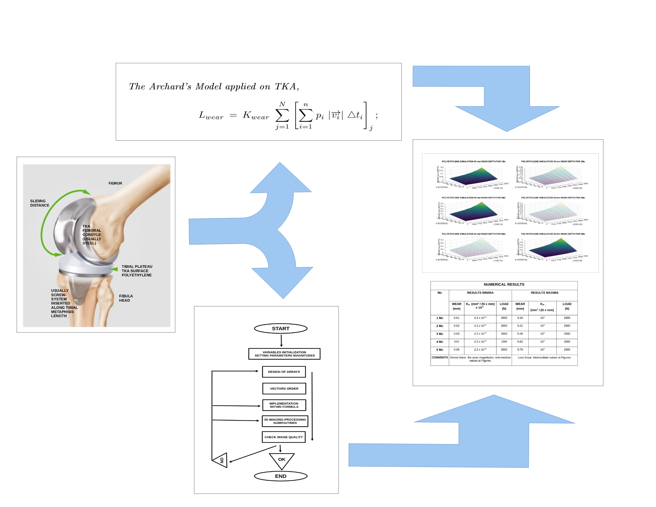
Primary approximations are to consider the TKA wear exclusively, and exclude Creep and Lubrication Factors (Equations (1) and (2)). Therefore, the calculations in this study provide a linear wear optimization approach to predict the durability of TKA implants using fundamental physical formulations [3,11]. Various models are applied in the literature (e.g., [22]); however, Archard’s model, with several variants, remains the most widely used [3,11]. Basic measurements taken into account in this study for in vitro and in vivo studies, including the contact area, correspond to [12-18]. Typical TKA wear values, most often obtained using the finite element method, are reported in [18-34]. Archard’s volume wear model (e.g., [23]) is not considered in the present study.

2.1. The basic Model Algorithm(s)

The basic algorithm-model from [3,11], as applied and analyzed, reads as follows:

$$\begin{array}{c}The Archard’s Model applied on TKA,\\ \hspace{1em}\hspace{1em}\hspace{1em}\hspace{1em}\hspace{1em}{L}_{wear}=K_{wear}{\displaystyle \sum _{j=1}^N}{\left[{\displaystyle \sum _{i=1}^n}{p}_i\right|\overrightarrow{v_i}|△t_i]}_j;\end{array}$$

(1)

where,

L_wear: Linear abrasive wear (mm).

K_wear: Wear constant, standard (mm³/N mm). Note: In the figures, the K_w values are typically multiplied by 10⁻³.

p_i: Pressure (N/mm²).

v_i: Sliding discrete Velocity for a discrete time increment (mm/s).

∆t_i: Discrete time interval (s).

i, j: Summatory indexes. The [i] is for velocity variation within a cycle (n). The [j] is for cycles number (N).

2.1.1. The Creep and Friction Factors

2.1.1.1. Creep

Although those factors are not applied in the study, descriptions with details of the Creep and Lubrication formulas are conveniently shown. For Creep [3], the model-equation format (Lee and Pienkowski, 1998) reads,

$$\begin{array}{c}\mathrm{The} \mathrm{Archard}’\mathrm{s} \mathrm{Model} \mathrm{complemented} \mathrm{with} \mathrm{Creep}, \mathrm{applied} \mathrm{on} \mathrm{TKA},\\ L_{total wear} = L_{linear wear} + L_{creep};\\ Hence,\\ L_{total wear} = L_{linear wear} \left[K_1+K_2\left(logt -4\right)\right] P_{average} h;\end{array}$$

(2)

where,

K₁: Model Constant [3]. The values for K₁ and K₂ are respectively, 3.491 × 10⁻³ and 7.961 × 10⁻⁴.

K₂: Model Constant [3]. The values for K₁ and K₂ are respectively, 3.491 × 10⁻³ and 7.961 × 10⁻⁴.

t: Time of load (minutes).

P_average: (N/mm²)

h: Polyethylene thickness (mm)

2.1.1.2. Friction

One common Friction Factor, set within the general formula is: [1 + 3 μ²]^½ [19-21], with values for UHWMPE of around [10⁻²] magnitude order. This Friction factor multiplies the general Formula (1) linearly. At this stage, it is not applied in the study. Friction was not set at this stage because the friction value in this case is approximately:

$${(1+3\times 0.072)}^{0.5}=1.0073,\left[\mathrm{a}\mathrm{dimensional}\right]$$

(2.1)

That is, an order of magnitude of 10⁻³. This implies that differences in magnitude, when applied within the algorithms, do not affect the order of significance. This level of precision is useful for further refinements.

2.1.2. The Integral Algorithm

When experimental data or a database is available, it is convenient to formulate the algorithm as an integral equation of the first kind. Accordingly, by taking appropriate limiting procedures, the problem can be expressed in integral form,

$$\begin{array}{c}\mathrm{The} \mathrm{Archard}’\mathrm{s} \mathrm{Model} \mathrm{applied} \mathrm{on} \mathrm{TKA}, \mathrm{integral} \mathrm{form},\\ L_{wear} = K_{wear} {\displaystyle \sum _{j=1}^N}{\displaystyle \sum _{i=1}^M} {\left[{\int }_0^{t_i}p \left|\overrightarrow{v}\right| dt\right]}_j ;\end{array}$$

(3)

where,

L_wear: Linear abrasive wear (mm).

K_wear: Wear constant, for programs (mm³/N mm). Note: at figures values range of K_w are usually multiplied by 10⁻³ because of this change of units (generally K_wear is formulated (mm³/N × m).

p(t): Instantaneous pressure (N/mm²). Function of time.

v(t): Instantaneous sliding velocity for integral. Function of time (mm/s).

dt: Differential of time during i-interval (s).

i; Summatory index for time at every integral for a cycle (M).

j; Summatory index for total cycles (N).

Proof 

The Archard’s Model applied on TKA, integral form proof,

For one cycle,

$$L_{w1}=K_{w}pS;$$

where S is sliding distance, hence

$$L_{w1}=K_{w}pvt;$$

therefore, provided $\overrightarrow{v}$ constant and taking derivatives for time variable,

$${\displaystyle \frac{d{L}_{w1}}{dt}}=K_{w}pv;or,$$

$$d{L}_{w1}=K_{w}pvdt,integrating,$$

$${\int }_0^{t}d{L}_{w1}=$$

$K_w{\int }_0^{t}pvdt$ , supposing instantaneous pressure and sliding velocity during one cycle,

Therefore, taking N cycles, and integrating,

$$L_{wear}=K_{wear}\sum _{j=1}^N\sum _{i=1}^M{[{\int }_0^{t_i},p_i,,\left|\overrightarrow{v_i}\right|,,d,t]}_j;$$

[Casesnoves Bioengineering Laboratory Algorithm 3114]

2.2. Computational Intelligence Dataset Software

The dataset selected from the literature spans a wide range of parameters, as the commercial materials, TKA sizes, and algorithmic constants employed vary across authors, laboratories, testing apparatuses, testing temperatures, and other experimental conditions. Therefore, the practical objective of the simulations-optimizations is to provide with large scale range that can be used to predict durability for all of those variants. The software is based on previous contributions by the authors in the development of hip wear programming and design [35,36]. A comprehensive biotribology database is available at [37-39].

2.2.1. Benchmark Polyethylene Model

Variations in TKA size have been reported across laboratory studies in the literature. However, the size used for simulation software implementation was the most standard one [1]. Specifically, a total coronal dimension of 78.2 × 44.2 mm was used, based on which the contact surface area was approximated and calculated. That size is according to ISO standards, and it is worth noting that there are ISO variants.

2.2.2. Sliding Distance (SD)

The sliding distance recommended by ISO is approximately 80 mm [10]. However, a value of 60 mm was adopted to account for differences in prosthesis sizes [12].

2.2.3. Load Magnitude

This is a magnitude convergence point for most of the studies. This is the magnitude most commonly assumed in the majority of investigations [19-21]. For example [2] (page 63), Table 1 and Table 2 provide an overview of the changes in loads and gait patterns from normal walking to descending stairs or ramps. Figure 1, Figure 2, Figure 3, Figure 4, Figure 5, Figure 6, Figure 7 and Figure 8 present comprehensive image-processing data. Based on this table and assuming an average patient weight of 75 kg, the range of loads corresponding to walking, stair descent, and stair ascent, among other activities, can be derived. Usually, then, it is [2000, 2600] N interval. Most simulation programs adopt a maximum load of 2300–2600 N. While some authors [19] use a maximum load of 3000 N, this value is not considered in the current study.

2.2.4. Standard Unit System

The linear wear of standard TKA, as predicted by Archard’s model, is typically expressed in the literature either as the volume of material removed (mm³) or as the erosion depth (mm) along the contact surface. When investigations are conducted in vivo or utilize cadaveric specimens, linear wear is commonly expressed in units of mm/year. Evaluating or determining the optimal unit system is not an objective of the present study. Instead, the image-processing and numerical data are expressed in millimeters of depth, allowing users to compare datasets appropriately [3,11]. The numerical comparative approximations constitute an important part of this study for the numerical dataset in mm/year. This is done by taking into account the average Mc for a year [16], which is about 2 Mc/year. The dimensional equations governing linear and volumetric abrasive wear are presented in (4).

2.2.5. Standard Abrasive Wear Kw Magnitude

Given the profusion of laboratory apparatus, measuring systems, and hybrid studies in the literature, there is no total agreement on the K_w magnitude [3]. Introduction: Figure 1 shows a 2D polynomial fit in GNU-Octave for imaging processing that describes the variation as a function of Kw and Million Cycles [13-23] integer interval. Note: the figure value range for K_w is usually multiplied by 10⁻³.

$$\begin{array}{l}Standard literature units for Archard’s model dimension equations,\\ For example,\\ \mathrm{Erosion} \mathrm{in} \mathrm{mm} \mathrm{depth},\\ L_w(mm depth)=K_w ({\displaystyle \frac{m{m}^3}{N mm}})Pressure ({\displaystyle \frac{N}{m{m}^2}}) Sliding Distance (mm);\\ as a result,L_w is in mm,\\ \mathrm{Erosion} \mathrm{in} {\mathrm{mm}}^3 \mathrm{eroded} \mathrm{material} \mathrm{volume},\\ V_w(m{m}^3 volume)=K_w ({\displaystyle \frac{m{m}^3}{N mm}})Pressure Force (N) Sliding Distance (mm);\\ as a result,V_w is in m{m}^3;\end{array}$$

(4)

The first method, which is the primary approach applied in this study, is abrasive linear wear.

2.3. Computational Intelligence Software

The software was developed primarily based on our previous experience with hip wear models [35,36]. The systems used were MATLAB® 2023 and GNU Octave® 7.1.0. For programming Equations (1) and (2), the difficulty was the matrix congruence and the loops for arrays.

3. Results and Discussion

Results are divided into Graphical and Numerical. In this primary stage, the numerical ones were determined by MATLAB graphical methods. The resolution of the 3D graphical optimization is acceptable, and the numerical results show approximate agreement with the standard literature [13-18]. Detailed numerical results are presented in Table 3, with comparative data summarized in Table 4.

Table 3:

Main numerical results in the study. Magnitudes match standard literature [13-18].

Numerical Results
Mc	Results Minima			Results Maxima
	Wear (mm)	KW (mm3/(N × mm) × 10−3	Load (Min Average) (N)	Wear (mm)	KW (mm3/(N × mm)	Load (Max Average) (N)
1 Mc	0.01	2.2 × 10−10	2000	0.16	10−9	2600
2 Mc	0.02	2.2 × 10−10	2000	0.31	10−9	2600
3 Mc	0.03	2.2 × 10−10	2000	0.46	10−9	2600
4 Mc	0.05	2.2 × 10−10	2000	0.62	10−9	2600
5 Mc	0.06	2.2 × 10−10	2000	0.78	10−9	2600
Comments	Almost linear wear magnitudes. Intermediate values at figures.			Less linear. Intermediate values at figures.

Table 4:

The main numerical results in the study. The wear magnitudes and rates differ in the literature and laboratories for two main reasons: (1) the large variety of testing apparatus and methods, including ISO variants, and (2) the large variety of ways to communicate/measure results. Namely, wear per Mc (mm), wear per year (mm), wear per Mc (mg), wear per year (mg), and others. In in vivo studies, wear is usually expressed in mm/year because the data are usually obtained from patients or recent cadaveric samples whose medical histories indicate the date of arthroplasty. What is common across the literature is that the polyethylene density is approximately equal to that of water. Magnitude orders match those in the standard literature [3, 11, 13-18]. An additional complementary dataset can be found at [19-34]. The FE method is generally for comparisons/validations with in vivo measurements. Computational optimization and general biotribology concepts are discussed in [35-38].

Comparative Numerical Results
Mc [Approx]	Results Approximated for All Comparisons Calculations, When In Vivo, It Is Taken from [16], an Average of 2 Mc By Year (Studies Differ Also)
	Author’s Study Linear Wear (mm)	1 [13, Hoshino and Alt, Wear + Creep, 2002] [In Vivo, 69 Patients, Geometrical Extrapolation]	2 [14, Teeter, m, and Alt, Wear + Creep, 2019] [In Vivo, 49 Patients] This Author Shows the Dataset for Maximum Wear, Lateral (Lat), and Medial (Med). It Is Shown [Ref], Lat = [0.034,0.069]/Year, and Med + [0.04,0.069]. All Angles.	3 [15, Gascoyne and Alt, Wear + Creep, 2019] [In Vivo, 106 Patients] This Author shows 0.015 mm/Year (Supine), and 0.220 mm/Year (Standing). The Proportional Average Set by the Author of This Study Is Calculated Here as: (4 × Standing + Supine)/5 = 0.1790. Approx = 0.18/Year.	4 [17, Ozer, Wear + Creep, 2022] [In Vivo-In-Vitro, FE Compared to 1 Cadaveric Sample, Flex + AP, Geometrical Extrapolation]
1 Mc	[0.01,0.16]	[0.001,0.01]	LAT [0.02, 0.03] MED [0.02,0.03]	[0.09]	[0.03]
2 Mc	[0.02,0.31]	[0.01,0.20]	LAT [0.03,0.07] MED [0.04,0.07]	[0.18]	[0.08]
3 Mc	[0.03,0.46]	[0.50,1.00]	LAT [0.07,0.09] MED [0.06,0.09]	[0.27]	[0.09]
4 Mc	[0.05,0.62]	[1.00,1.10]	LAT [0.08,0.12] MED [0.08,0.12]	[0.36]	[0.10]
5 Mc	[0.06,0.78]	[1.10,1.20]	LAT [0.10,0.15] MED [0.10,0.15]	[0.45]	[0.13]
Comments	Almost linear wear magnitudes when the Mc number is low, proportional to the Mc number. Differences tend to become nonlinear as a function of Mc when the Mc magnitude increases.
Important Disclaimer	The wear magnitudes and rates differ in literature and laboratories for two main reasons: (1) The large variety of testing apparatus and methods, (2) the large variety to communicate/measureresults. Namely, Wear Per Mc (mm), Wear Per Year (mm), Wear Per Mc (mg), Wear Per Year (mg), and others. When the study is in vivo, Wear is usually expressed in mm/year. What is common is the polyethylene density approximately equal to water.

3.1. 3D Graphical Optimization Results

The linear wear graphical optimization method presented here builds upon our earlier publications on volumetric wear in hip arthroplasty [35,36]. It essentially consists of finding the global/local minima by using the 3D imaging surfaces of the algorithm’s objective function, plus two selected parameters. The method is applied to wear formulas (1) and (2) to identify optimal minima or target values under particular constraints across the 3D surface. Illustrative Example 1 demonstrates the initiation of this procedure. Initially, tentative programs are developed. Once the software functionality and numerical consistency of the 3D graphs are verified, the final 3D graphical optimization image-processing charts are generated using accurate parameters and intervals. Note: in the figures, the values along the Kw axis are often multiplied by 10−3 because of the units. Figure 4, Figure 5, Figure 6, Figure 7, Figure 8 and Figure 9 show all the Graphical Optimization results for the dataset. Figure 10, Figure 11, Figure 12 and Figure 13 show extensive image processing of the results. The main references suggested for the reader to gain knowledge of computational intelligence software are useful [35-36, 40-62]. Precise programming charts can be found in the cited references. For further study, references [55-60] offer additional insights into polymer materials, biomechanics, and tribology and are recommended to the reader.

3.2. Numerical Results

Table 3 presents the numerical results for linear wear extracted from the graphical optimization. In Table 4, the figures and corresponding magnitudes are compared with values reported in the standard literature [13-18]. For orthopedics, wear implants, and general software, it is recommended to consult [35-36, 40-62]. Figure 4, Figure 5, Figure 6, Figure 7, Figure 8 and Figure 9 show all the Graphical Optimization results for the dataset. The references [57-62] are intended as complementary further reading on polymer materials, biomechanics, and tribology and are recommended for the reader.

3.3. Comparison of Numerical Results

Table 4 presents some numerical comparisons with other literature studies. Some of them are carried out with the FE Method, and others with the FE Method and contrasted with cadaveric data. The most important objective consequence is that from [2,3] Mc on, the Linear Erosion shows a magnitude order jump from 10⁻² to 10⁻¹ mm. The comparisons are shown for the database from [13-17]. However, a more extensive database is available at [18-34].

3.4. Biomaterials and Biomechanics TKA Applications Briefing

Table 5 shows a concise concept of study applications. The most important aspect is the prediction of erosion rates, which provides approximations for implant durability [37-57, 63-81]. Several additional applications can be inferred from Table 5.

Table 5:

Biomechanical and Biotribological applications briefing. Some of them are similar to previous studies in hip joint wear [35,36].

Applications Briefing
Principal Utility in Computational Bioengineering	TKA Wear Predictions and efficacious calculations at 3D image-processing graphs, especially with MATLAB, to know the exact magnitude for any selected KW and Load (x, y, coordinates), the approximate abrasive wear magnitude for 1–5 Mc.
Wear and Biotribology Predictions	For the design/manufacturing of TKA prostheses. This is the most important utility. TKA erosion prediction, especially for polyethylene materials, is essential. Prediction saves manufacturing-research time, reduces the need to repeat laboratory work, and saves budget.
TKA Durability Prediction	To provide patients with a quality of life. To avoid re-operations and substitution for new prostheses.
Industrial Manufacturing	Optimization of the manufacturing process and improvement of quality.
I + D Research	The TKA prostheses are continually evolving. For the future design of new types. Similar/variants of materials I + D.
Patient Life Quality	Very important for the normal movement of the patient. Walking and essential movements are easy and comfortable for the patient during the entire duration.
Sport Medicine	This is a very important application because sports medicine requires these prostheses in higher quality than common patients.

4. Conclusions

5. Future Developments

List of Abbreviations

Author Contributions

Availability of Data and Materials

Conflicts of Interest

Funding

Acknowledgments

AI Declaration

References

[1] Dawim, P. (Ed.) Biomaterials and Medical Tribology: Research and Development; Woodhead Publishing: Cambridge, UK, 2013; Available online: https://www.sciencedirect.com/book/edited-volume/9780857090171/biomaterials-and-medical-tribology.

[2] Schaldach, M.; Hohmann, D. Advances in Artificial Hip and Knee Joint Technology; Springer: Berlin/Heidelberg, Germany, 1976; Available online: https://link.springer.com/book/10.1007/978-3-642-66369-7.

[3] Jin, Z. Computational Modelling of Biomechanics and Biotribology in the Musculoskeletal System; Woodhead Publishing: Cambridge, UK, 2014. [CrossRef]

[4] Munzinger, U.; Boldt, J.; Keblish, P. Primary Knee Arthroplasty; Springer: Berlin/Heidelberg, Germany, 2004. [CrossRef]

[5] Dawim, P.J. Biotribology; Wiley: Hoboken, NJ, USA, 2010; Available online: https://www.wiley.com/en-us/Biotribology-p-9781848212756.

[6] Sculco, T.; Martucci, E. (Eds.) Knee Arthroplasty; Springer: Vienna, Austria, 2001. [CrossRef]

[7] Tokgoz, E.; Levitt, S.; Sosa, D.; Carola, N.A.; Patel, V. Total Knee Arthroplasty: A Review of Medical and Biomedical Engineering and Science Concepts; Springer: Berlin/Heidelberg, Germany, 2023. [CrossRef]

[8] Kumar, A.; Kumar, A.; Kumar, A. (Eds.) Applications of Biotribology in Biomedical Systems; Springer: Cham, Switzerland, 2024. [CrossRef]

[9] Kretzer, J. Wear in Total Knee Arthroplasty—Just a Question of Polyethylene? Int. Orthopaedics (SICOT) 2014, 38, 335–340. [CrossRef]

[10] D’Lima, D. In Vivo Tibial Force Measurement after Total Knee Arthroplasty. Ph.D. Thesis, University of California San Diego Electronic Theses and Dissertations, San Diego, CA, USA, 2007. Available online: https://escholarship.org/uc/item/7xd465w1.

[11] Affatato, S. Wear of Orthopaedic Implants and Artificial Joints; Woodhead Publishing: Cambridge, UK, 2012; Available online: https://www.sciencedirect.com/book/edited-volume/9780857091284/wear-of-orthopaedic-implants-and-artificial-joints.

[12] Triwardono, J.; Supriadi, S.; Whulanza, Y.; Saragih, A.S.; Novalianita, D.A.; Utomo, M.S.; Kartika, I. Evaluation of the Contact Area in Total Knee Arthroplasty Designed for Deep Knee Flexion. Int. J. Technol. 2021, 12, 1312–1322. [View Online]

[13] Hoshino, A.; Fukuoka, Y.; Ishida, A. Accurate In Vivo Measurement of Polyethylene Wear in Total Knee Arthroplasty. J. Arthroplast. 2002, 17, 490–496. [CrossRef]

[14] Teeter, M.G.; Wihlidal, J.; McCalden, R.W.; Yuan, X.; MacDonald, S.J.; Lanting, B.A.; Naudie, D.D. Radiostereometric Analysis Permits In Vivo Measurement of Very Small Levels of Wear in TKA. Clin. Orthop. Relat. Res. 2019, 477, 80–90. [CrossRef]

[15] Gascoyne, T.; Parashin, S.; Teeter, M.; Bohm, E.; Laende, E.; Dunbar, M.; Turgeon, T. In Vivo Wear Measurement in a Modern Total Knee Arthroplasty with Model-Based Radiostereometric Analysis. Bone Jt. J. 2019, 101-B, 1348–1355. [CrossRef]

[16] Silva, M.; Shepherd, E.F.; Jackson, W.O.; Dorey, F.J.; Schmalzried, T.P. Average Patient Walking Activity Approaches 2 Million Cycles per Year: Pedometers Under-Record Walking Activity. J. Arthroplast. 2002, 17, 693–697. [CrossRef]

[17] Ozer, A. Computational Wear of Knee Implant Polyethylene Insert Surface under Continuous Dynamic Loading and Posterior Tibial Slope Variation Based on Cadaver Experiments with Comparative Verification. BMC Musculoskelet. Disord. 2022, 23, 871. [CrossRef]

[18] Heisel, C.; Silva, M.; dela Rosa, M.A.; Schmalzried, T.P. Short-Term In Vivo Wear of Cross-Linked Polyethylene. J. Bone Jt. Surg. 2004, 86. [CrossRef] [PubMed]

[19] Soni, A. Total Knee Arthroplasty (TKA) Wear Analysis on the Tibial Implant Using Finite Element Method Approach. Int. J. All Res. Educ. Sci. Methods 2020, 6. [View Online]

[20] Bergmann, G.; Bender, A.; Graichen, F.; Dymke, J.; Rohlmann, A.; Trepczynski, A.; Heller, M.O.; Kutzner, I. Standardized Loads Acting in Knee Implants. PLoS ONE 2014, 9, e86035. [CrossRef] [PubMed]

[21] Dreyer, M.J.; Trepczynski, A.; Nasab, S.H.H.; Kutzner, I.; Schütz, P.; Weisse, B.; Dymke, J.; Postolka, B.; Moewis, P.; Bergmann, G.; et al. European Society of Biomechanics S.M. Perren Award 2022: Standardized Tibio-Femoral Implant Loads and Kinematics. J. Biomech. 2022, 141, 111171. [CrossRef]

[22] Abdelgaied, A.; Liu, F.; Brockett, C.; Jennings, L.; Fisher, J.; Jin, Z. Computational Wear Prediction of Artificial Knee Joints Based on a New Wear Law and Formulation. J. Biomech. 2011, 44, 1108–1116. [CrossRef]

[23] Pecora, J.; Romero, V. Evaluation of Polyethylene Wear in a Brazilian Ultracongruent Knee Prosthesis with a Rotating Platform. Rev. Bras. Ortop. 2021, 56, 42–46. [CrossRef]

[24] Innocenti, B.; Labey, L.; Kamali, A.; Pascale, W.; Pianigiani, S. Development and Validation of a Wear Model to Predict Polyethylene Wear in a Total Knee Arthroplasty: A Finite Element Analysis. Lubricants 2014, 2, 193–205. [CrossRef]

[25] De Ruiter, L.; Cowie, R.M.; Jennings, L.M.; Briscoe, A.; Janssen, D.; Verdonschot, N. The Effects of Cyclic Loading and Motion on the Implant–Cement Interface and Cement Mantle of PEEK and Cobalt–Chromium Femoral Total Knee Arthroplasty Implants: A Preliminary Study. Materials 2020, 13, 3323. [CrossRef]

[26] Kumar, V.; Tewari, R.P.; Pandey, R.; Rawat, A. Triboinformatic Modeling of Wear in Total Knee Replacement Implants Using Machine Learning Algorithms. J. Mater. Eng. 2023, 1, 97–105. [CrossRef]

[27] Fishera, J.; McEwen, H.M.J.; Barnett, P.I.; Bell, C.J.; Stewart, T.D.; Stone, M.H.; Ingham, E. Wear of Polyethylene in Artificial Knee Joints. Curr. Orthop. 2001, 15, 399–405. [CrossRef]

[28] Fuchs, S.; Schütte, G.; Witte, H.; Rosenbaum, D. Retropatellar Contact Characteristics in Total Knee Arthroplasty with and without Patellar Resurfacing. Int. Orthopaedics (SICOT) 2000, 24, 191–193. [CrossRef] [PubMed]

[29] Koh, Y.G.; Park, K.M.; Lee, H.Y.; Park, J.H.; Kang, K.T. Prediction of Wear Performance in Femoral and Tibial Conformity in Patient-Specific Cruciate-Retaining Total Knee Arthroplasty. J. Orthop. Surg. Res. 2020, 15, 24. [CrossRef]

[30] Stukenborg-Colsman, C.; Ostermeier, S.; Hurschler, C.; Wirth, C.J. Tibiofemoral Contact Stress after Total Knee Arthroplasty. Acta Orthop. Scand. 2002, 73, 638–646. [CrossRef]

[31] Uvehammer, J. Knee Joint Kinematics, Fixation and Function Related to Joint Area Design in Total Knee Arthroplasty. Acta Orthop. Scand. Suppl. 2001, 72, 1–52. [CrossRef]

[32] Abdelgaied, A.A.; Fisher, J.; Jennings, L. Understanding the Differences in Wear Testing Method Standards for Total Knee Replacement. J. Mech. Behav. Biomed. Mater. 2022, 132, 105258. [CrossRef]

[33] Dai, Y.; Scuderi, G.R.; Penninger, C.; Bischoff, J.E.; Rosenberg, A. Increased Shape and Size Offerings of Femoral Components Improve Fit during Total Knee Arthroplasty. Knee Surg. Sports Traumatol. Arthrosc. 2014, 22, 2931–2940. [CrossRef]

[34] Fekete, G.; Sun, D.; Gu, Y.; Neis, P.D.; Ferreira, N.F.; Innocenti, B.; Csizmadia, B.M. Tibiofemoral Wear in Standard and Non-Standard Squat: Implication for Total Knee Arthroplasty. Muscles Ligaments Tendons J. 2017, 7, 520–528. [PubMed]

[35] Casesnoves, F. Multiobjective Optimization for Ceramic Hip Arthroplasty with Medical Physics Applications. Int. J. Sci. Res. Comput. Sci. Eng. Inf. Technol. 2021, 7, 582–598. [CrossRef]

[36] Casesnoves, F. Nonlinear Comparative Optimization for Biomaterials Wear in Artificial Implants Technology. In Proceedings of the Applied Chemistry and Materials Science RTU2018 Conference, Riga, Latvia, 26 October 2018. [CrossRef]

[37] Merola, M.; Affatato, S. Materials for Hip Prostheses: A Review of Wear and Loading Considerations. Materials 2019, 12, 495. [CrossRef]

[38] Navarro, N. Biomaterials in Orthopaedics. J. R. Soc. Interface 2008, 5, 1137–1158. [CrossRef] [PubMed]

[39] Sachin, G.; Mankar, A.; Bhalerao, Y. Biomaterials in Hip Joint Replacement. Int. J. Mater. Sci. Eng. 2016, 4, 113–125. [View Online]

[40] Casesnoves, F. 2D Computational-Numerical Hardness Comparison between Fe-Based Hardfaces with WC-Co Reinforcements for Integral-Differential Modelling. Solid State Phenom. 2018, 762, 330–338. [CrossRef]

[41] Casesnoves, F.; Antonov, M.; Kulu, P. Mathematical Models for Erosion and Corrosion in Power Plants: A Review of Applicable Modelling Optimization Techniques. In Proceedings of the RUTCON2016 Power Engineering Conference, Riga, Latvia, 13 October 2016. Available online: https://ieeexplore.ieee.org/document/7763117.

[42] Casesnoves, F. The Numerical Reuleaux Method: A Computational and Dynamical Base with Applications. First Part; Lambert Academic Publishing: Saarland, Germany, 2019; ISBN 103659917478. Available online: https://www.cede.ch/en/books/francisco-casesnoves-the-numerical-reuleaux-method-computational-and-dynamical-f-154504999.

[43] Kulo, P.; Casesnoves, F.; Simson, T.; Tarbe, R. Prediction of Abrasive Impact Wear of Composite Hardfacings. Solid State Phenom. 2017, 267, 201–206. [CrossRef]

[44] Casesnoves, F. Mathematical Models and Optimization of Erosion and Corrosion. Ph.D. Thesis, Taltech University, Tallinn, Estonia, 2018. Available online: https://digikogu.taltech.ee/et/item/714f5c22-f74b-4d18-af83-969ca0410aac.

[45] Casesnoves, F. Large-Scale Matlab Optimization Toolbox (MOT) Computing Methods in Radiotherapy Inverse Treatment Planning. In High Performance Computing Meeting; Nottingham University: Nottingham, UK, 2007.

[46] Casesnoves, F. A Monte-Carlo Optimization Method for the Movement Analysis of Pseudo-Rigid Bodies. In Proceedings of the 10th SIAM Conference in Geometric Design and Computing, San Antonio, TX, USA, 4–8 November 2007. Available online: https://scholar.google.com/scholar?q=A+MonteCarlo+Optimization+Method+for+the+Movement+Analysis+of+Pseudo-Rigid+Bodies+Casesnoves+2007.

[47] Casesnoves, F. Theory and Primary Computational Simulations of the Numerical Reuleaux Method (NRM). Int. J. Math. Comput. 2011, 13, 89-D11. [View Online]

[48] Casesnoves, F. Applied Inverse Methods for Optimal Geometrical-Mechanical Deformation of Lumbar Artificial Disks/Implants with Numerical Reuleaux Method: 2D Comparative Simulations and Formulation. Comput. Sci. Appl. 2015, 2, 1–10. [View Online]

[49] Casesnoves, F. Inverse Methods and Integral-Differential Model Demonstration for Optimal Mechanical Operation of Power Plants–Numerical Graphical Optimization for Second Generation of Tribology Models. Electr. Control Commun. Eng. 2018, 14, 39–50. [CrossRef]

[50] Casesnoves, F.; Surzhenkov, A. Inverse Methods for Computational Simulations and Optimization of Erosion Models in Power Plants. In Proceedings of the IEEE Proceedings of RUTCON2017 Power Engineering Conference, Riga, Latvia, 5 December 2017. [CrossRef]

[51] Casesnoves, F. Exact Integral Equation Determination with 3D Wedge Filter Convolution Factor Solution in Radiotherapy: Series of Computational-Programming 2D–3D Dosimetry Simulations. Int. J. Sci. Res. Sci. Eng. Technol. 2016, 2, 699–715. [View Online]

[52] Casesnoves, F. Software Programming with Lumbar Spine Cadaveric Specimens for Computational Biomedical Applications. Int. J. Sci. Res. Comput. Sci. Eng. Inf. Technol. 2021, 7, 7–13. [CrossRef]

[53] Surzhenkov, A.; Viljus, M.; Simson, T.; Tarbe, R.; Saarna, M.; Casesnoves, F. Wear Resistance and Mechanisms of Composite Hardfacings at Abrasive Impact Erosion Wear. J. Phys. Conf. Ser. 2017, 843, 012060. [CrossRef]

[54] Casesnoves, F. Computational Simulations of Vertebral Body for Optimal Instrumentation Design. ASME J. Med. Devices 2012, 6, 021014. [CrossRef]

[55] Barker, P. The Effect of Applying Tension to the Lumbar Fasciae on Segmental Flexion and Extension. In Proceedings of the 5th International Congress of Low Back and Pelvic Pain, Melbourne, Australia, 10–13 November 2014; pp. 50–52. Available online: https://scholar.google.com/scholar?q=Effect+of+Applying+Tension+to+the+Lumbar+Fasciae+Barker.

[56] European Commission, Directorate-General for Research. European Textbook on Ethics in Research. EUR 24452 EN. Available online: https://op.europa.eu/en/publication-detail/-/publication/12567a07-6beb-4998-95cd-8bca103fcf43 (accessed on 28 June 2021).

[57] ALLEA. The European Code of Conduct for Research Integrity, Revised ed.; ALLEA: Berlin, Germany, 2017; Available online: https://allea.org/european-code-of-conduct-2017/

[58] Bains, P.S.; Singh, G.; Bhui, A.S.; Sidhu, S.S.; Bains, P. Biomaterials in Orthopaedics and Bone Regeneration; Springer: Berlin/Heidelberg, Germany, 2019. [CrossRef]

[59] Stergiou, N. Biomechanics and Gait Analysis; Academic Press: Cambridge, MA, USA, 2020; Available online: https://www.sciencedirect.com/book/monograph/9780128133729/biomechanics-and-gait-analysis.

[60] Tanzi, M.; Fare, S. Characterization of Polymeric Biomaterials; Woodhead Publishing: Cambridge, UK, 2021. [CrossRef]

[61] Okuno, E.; Fratin, L. Biomechanics of the Human Body; Springer: Berlin/Heidelberg, Germany, 2014. [CrossRef]

[62] Abhilash, P.; Kumar, K.; Gajrani; Luo, X. Bioimplants Manufacturing; CRC Press: Boca Raton, FL, USA, 2025. [CrossRef]

[63] Kurtz, S. Advances in Zirconia Toughened Alumina Biomaterials for Total Joint Replacement. J. Mech. Behav. Biomed. Mater. 2014, 31, 107–116. [CrossRef]

[64] Li, Y.; Yang, C.; Zhao, H.; Qu, S.; Li, X.; Li, Y. New Developments of Ti-Based Alloys for Biomedical Applications. Materials 2014, 7, 1709–1800. [CrossRef]

[65] Kolli, R.; Devaraj, A. A Review of Metastable Beta Titanium Alloys. Metals 2018, 8, 506. [CrossRef]

[66] Holzwarth, U.; Cotogno, G. Total Hip Arthroplasty; European Commission: Brussels, Belgium, 2012; JRC Scientific and Policy Reports. [CrossRef]

[67] Delimar, D. Femoral Head Wear and Metallosis Caused by Damaged Titanium Porous Coating after Primary Metal-on-Polyethylene Total Hip Arthroplasty: A Case Report. Croat. Med. J. 2018, 59, 253–257. [CrossRef]

[68] Zhang, M.; Fan, Y. Computational Biomechanics of the Musculoskeletal System; CRC Press: Boca Raton, FL, USA, 2015. [CrossRef]

[69] Dreinhöfer, K.; Dieppe, P.; Günther, K.; Puhl, W. Eurohip: Health Technology Assessment of Hip Arthroplasty in Europe; Springer: Berlin/Heidelberg, Germany, 2009. [CrossRef]

[70] Hutchings, I.; Shipway, P. Tribology: Friction and Wear of Engineering Materials, 2nd ed.; Elsevier: Amsterdam, The Netherlands, 2017; Available online: https://www.sciencedirect.com/book/monograph/9780081009109/tribology.

[71] Shen, X.; Lei, C.; Li, R. Numerical Simulation of Sliding Wear Based on Archard Model. In Proceedings of the 2010 International Conference on Mechanic Automation and Control Engineering, Wuhan, China, 26–28 June 2010. [CrossRef]

[72] Affatato, S.; Brando, D. Introduction to Wear Phenomena of Orthopaedic Implants; Woodhead Publishing: Sawston, UK, 2012. [CrossRef]

[73] Matsoukas, G.; Kim, Y. Design Optimization of a Total Hip Prosthesis for Wear Reduction. J. Biomech. Eng. 2009, 131, 051003. [CrossRef] [PubMed]

[74] Galante, J.; Rostoker, W. Wear in Total Hip Prostheses. Acta Orthop. Scand. 2014, 43, 1–46. [CrossRef] [PubMed]

[75] Mattei, L.; DiPuccio, F.; Piccigallo, B.; Ciulli, E. Lubrication and Wear Modelling of Artificial Hip Joints: A Review. Tribol. Int. 2011, 44, 532–549. [CrossRef]

[76] Jennings, L. Enhancing the Safety and Reliability of Joint Replacement Implants. Orthop. Trauma 2012, 26, 246–252. [CrossRef]

[77] Saifuddin, A.; Blease, S.; Macsweeney, E. Axial Loaded MRI of the Lumbar Spine. Clin. Radiol. 2003, 58, 661–671. [CrossRef]

[78] Damm, P. Loading of Total Hip Joint Replacements. Ph.D. Thesis, Technischen Universität, Berlin, Germany, 2014. [CrossRef]

[79] Abramowitz, S. Handbook of Mathematical Functions; National Bureau of Standards: Gaithersburg, MD, USA, 1972; Applied Mathematics Series • 55, Library of Congress Catalog Card Number: 64:-60036. Available online: https://personal.math.ubc.ca/~cbm/aands/frameindex.htm.

[80] Luenberger, G.D. Linear and Nonlinear Programming, 4th ed.; Springer: Berlin/Heidelberg, Germany, 2008. [CrossRef]

[81] Panjabi, M.; White, A. Clinical Biomechanics of the Spine; Lippincott: New York, NY, USA, 1980; Available online: https://www.academia.edu/120640431/Clinical_Biomechanics_of_the_Spine.